决策树及其在手写数字识别的实践

引言

决策时是一种基本的分类和回归方法，现在主要讨论分类决策树。决策树模型呈树形结构，在分类问题中，表示基本特征对实例进行分类的过程，你可以认为他是一个 if-then 的集合，也可以认为是定义在特征空间与类空间上的条件概率分布。

其优点是模型具有可读性，分类速度快，学习时，利用训练数据，根据损失函数最小化的原则建立决策树模型。预测的时，对新的数据利用训练建立的决策树模型来分类。

决策树学习分为三个步骤：特征选择、决策树生成和决策树的剪枝。主要的决策树生成算法有 ID3 算法、C4.5 算法、 CART 算法。

本文的大纲如下：

1. 介绍决策树模型的基本概念
2. 决策树的特征选择和学习过程
3. 以 ID3 算法为例进行手写数字识别实践

决策树模型的基本概念

决策树模型

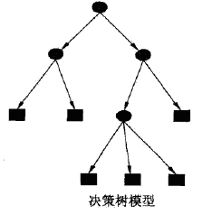
分类决策树是一种描述对实例进行分类的树形结构。决策树由节点和有向边组成，节点分为两类：内部结点和叶节点。内部结点表示一个特征或者属性，叶节点表示一个分类。

用决策树分类的过程类似于一系列的 if-then 判断，如下图的一个决策树，圆和方框分别表示内部节点和叶节点，决策分类过程是这样的：首先从顶端的根节点出发，每个内部结点都是一个特征判断，即是 if-then 判断，如果满足特征是一种路径，不满足特征是另一条路径。

决策树学习

决策树学习，假设给定训练数据集：

$$D=\{(x_1,y_1),(x_2,y_2),\cdots,(x_N,y_N)\}$$

其中，$x_i = (x_i^1,x_i^2,\cdots,x_i^n)$ 为输入实力（特征向量），n为特征个数， $y_i\in\{1,2,\cdots,K\}$为类标记，$i=1,2,\cdots,N$，N 为样本容量。学习的目标是根据给定的训练数据集构建一个决策树模型，使他能够进行正确的分类。

而通过上面决策树的概念介绍，我们可以知道，决策树学习本质上是从训练数据集中归纳出一组分类规则。与训练数据集不相矛盾的决策树（即是能对训练数据进行正确分类的决策树）可能有多个，有可能一个都没有。我们需要的是一个与训练数据矛盾较小的决策树，同时有较好的泛化能力。

决策树学习的损失函数通常是正则化的极大似然函数。决策树学习的策略也自然是以损失函数为目标函数的最小化。而这是一个 NP 问题，所以一般采用启发式的方法求得一个次最优解。

决策树学习的算法通常是一个递归的选择最优特征，并根据该特征对训练数据进行分割，使得对各个子数据集有一个最好的分类的过程。

特征选择

特征选择在于选取对训练数据具有分类能力的特征，这样可以提高决策树学习的效率，而衡量特征分类效果的函数就是信息增益函数。

信息增益

信息增益是信息论中的概念，了解信息增益，首先要了解熵和条件熵的定义。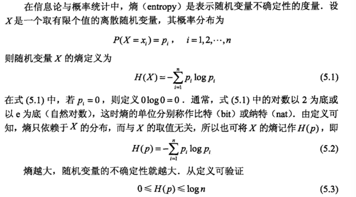

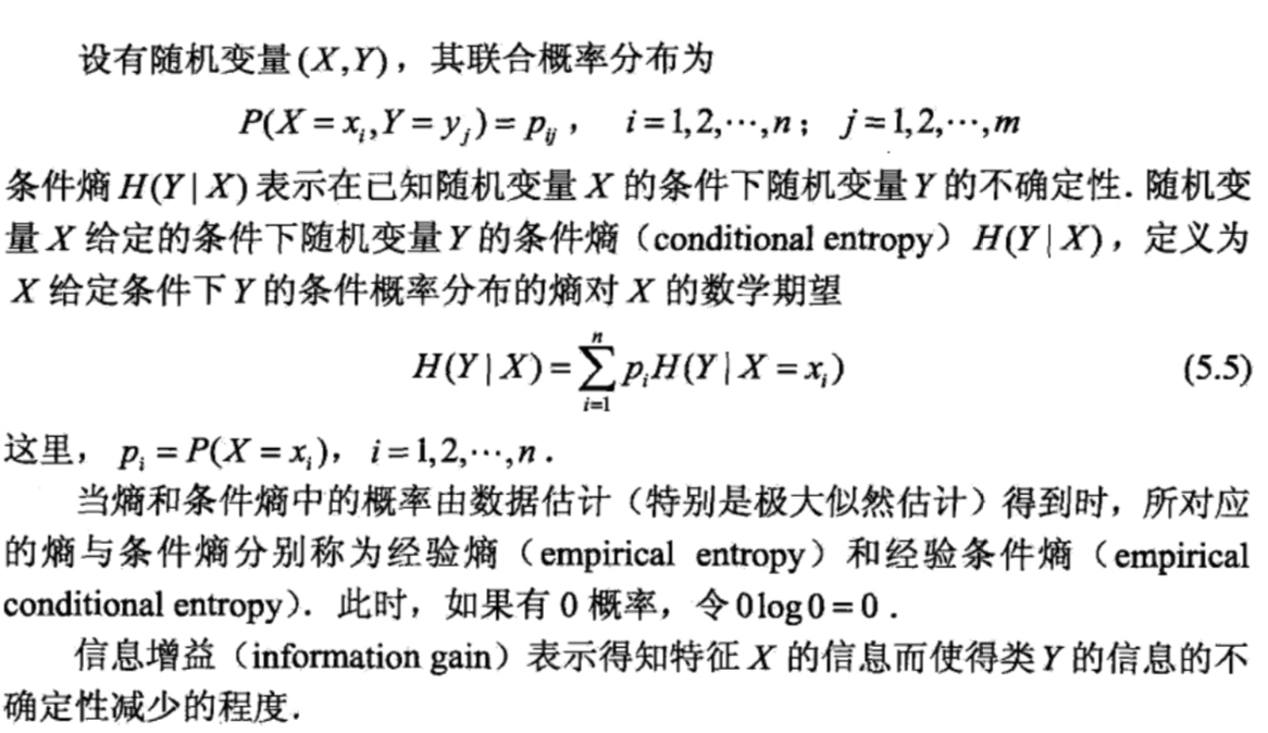
信息增益的定义：特征 A 对训练集 D 对信息增益 g(D,A)，定义为集合 D 的经验熵 H(D) 与特征 A 给定的条件下 D 的经验条件熵 H(D|A) 之差，即是：

$$g(D,A) = H(D)-H(D|A)$$

信息增益算法

• 基本假设
  

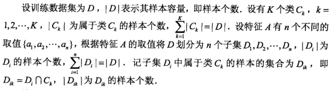
于是信息增益算法如下：
输入：训练数据集 D 和特征 A；
输出：特征 A 对训练数据集 D 的信息增益 g(D,A)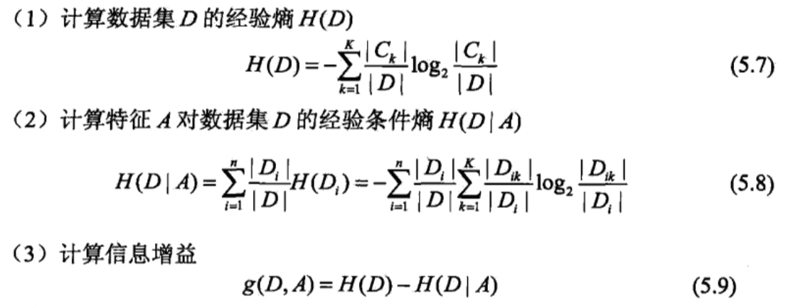

决策树生成

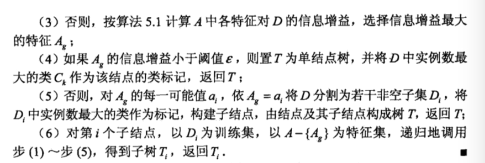
ID3 算法的核心是在决策树各个节点上应用信息增益准则选择特征，递归的构建决策树。具体点方法是：从根结点开始，对节点计算所有可能的特征的信息增益，选择信息增益最大的特征作为节点的特征，由该特征的不同取值建立子节点；再对子节点递归的调用以上方法，构建决策树；知道所有的特征的信心增益均很小或者没有特征可以选择为止。最后得到一个决策树，ID3 算法相当于用最大似然估计进行概率模型的选择。

ID3 算法

输入：训练数据 D，特征集 A，阈值 $\epsilon$
输出：决策树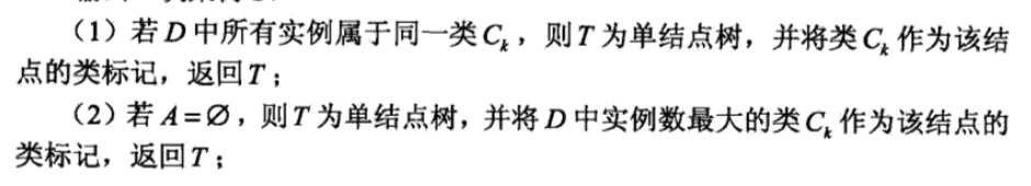

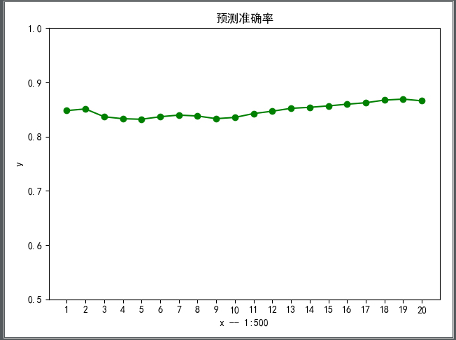
ID3 算法只有树的生成，所以其生成的树很容易过拟合。

以下为该算法的代码在 Mnist 数据集上实现的准确率，86.7%，比不上 KNN 的准确度，但是速度比其快的多。

代码如下：

#encoding=utf-8

import cv2
import time
import logging
import numpy as np
import matplotlib.pyplot as plt
import testLibrary as tl


ALL_DATA = 60000

total_class = 10


def log(func):
    def wrapper(*args, **kwargs):
        start_time = time.time()
        logging.debug('start %s()' % func.__name__)
        ret = func(*args, **kwargs)

        end_time = time.time()
        logging.debug('end %s(), cost %s seconds' % (func.__name__,end_time-start_time))

        return ret
    return wrapper


# 二值化
def binaryzation(img):
    cv_img = img.astype(np.uint8)
    cv2.threshold(cv_img,50,1,cv2.cv.CV_THRESH_BINARY_INV,cv_img)
    return cv_img


@log
def binaryzation_features(trainset):
    features = []

    for img in trainset:
        img = np.reshape(img,(28,28))
        cv_img = img.astype(np.uint8)

        img_b = binaryzation(cv_img)
        # hog_feature = np.transpose(hog_feature)
        features.append(img_b)

    features = np.array(features)
    features = np.reshape(features, (-1, 784))

    return features


class Tree(object):
    def __init__(self, node_type, Class=None, feature=None):
        self.node_type = node_type
        self.dict = {}
        self.Class = Class
        self.feature = feature

    def add_tree(self, val, tree):
        self.dict[val] = tree

    def predict(self, features):
        if self.node_type == 'leaf':
            return self.Class

        tree = self.dict[features[self.feature]]
        return tree.predict(features)


def calc_ent(x):
    """
        calculate shanno ent of x
    """

    x_value_list = set([x[i] for i in range(x.shape[0])])
    ent = 0.0
    for x_value in x_value_list:
        p = float(x[x == x_value].shape[0]) / x.shape[0]
        logp = np.log2(p)
        ent -= p * logp
    return ent


def calc_condition_ent(x, y):
    """
        calculate ent H(y|x)
    """

    # calc ent(y|x)
    x_value_list = set([x[i] for i in range(x.shape[0])])
    ent = 0.0
    for x_value in x_value_list:
        sub_y = y[x == x_value]
        temp_ent = calc_ent(sub_y)
        ent += (float(sub_y.shape[0]) / y.shape[0]) * temp_ent

    return ent

#
# def calc_ent_grap(x,y):
#     """
#         calculate ent grap
#     """
#     base_ent = calc_ent(y)
#     condition_ent = calc_condition_ent(x, y)
#     ent_grap = base_ent - condition_ent
#
#     return ent_grap

def recurse_train(train_set, train_label, features, epsilon):
    global total_class

    LEAF = 'leaf'
    INTERNAL = 'internal'

    # 步骤1——如果train_set中的所有实例都属于同一类Ck
    label_set = set(train_label)
    if len(label_set) == 1:
        return Tree(LEAF, Class=label_set.pop())

    # 步骤2——如果features为空
    (max_class, max_len) = max([(i, len([x for x in train_label if x == i])) for i in range(total_class)],key = lambda x:x[1])

    if len(features) == 0:
        return Tree(LEAF, Class=max_class)

    # 步骤3——计算信息增益
    max_feature = 0
    max_gda = 0

    d = train_label
    hd = calc_ent(d)
    for feature in features:
        A = np.array(train_set[:, feature].flat)
        gda = hd - calc_condition_ent(A, d)

        if gda > max_gda:
            max_gda, max_feature = gda, feature

    # 步骤4——小于阈值
    if max_gda < epsilon:
        return Tree(LEAF, Class=max_class)

    # 步骤5——构建非空子集
    sub_features = [x for x in features if x != max_feature]
    tree = Tree(INTERNAL, feature=max_feature)

    feature_col = np.array(train_set[:, max_feature].flat)
    feature_value_list = set([feature_col[i] for i in range(feature_col.shape[0])])
    for feature_value in feature_value_list:

        index = []
        for i in range(len(train_label)):
            if train_set[i][max_feature] == feature_value:
                index.append(i)

        sub_train_set = train_set[index]
        sub_train_label = train_label[index]

        sub_tree = recurse_train(sub_train_set,sub_train_label,sub_features,epsilon)
        tree.add_tree(feature_value,sub_tree)

    return tree


@log
def train(train_set, train_label, features, epsilon):
    return recurse_train(train_set, train_label, features, epsilon)


@log
def predict(test_set, tree):

    result = []
    for features in test_set:
        tmp_predict = tree.predict(features)
        result.append(tmp_predict)
    return np.array(result)


def calculate_accuracy(predict_ary, test):
    right_count = 0.0
    accuracy_ary = []
    for index in range(len(predict_ary)):
        if predict_ary[index] == test[index]:
            right_count += 1
            if (index + 1) % 500 == 0:
                accuracy_ary.append(float(right_count) / (index + 1))
        print("预测值：%d 实际值： %d" % (predict_ary[index], test[index]))
    return right_count/len(test), accuracy_ary


if __name__ == '__main__':
    logger = logging.getLogger()
    logger.setLevel(logging.DEBUG)

    # 读取训练数据集和测试数据集的方法和朴素贝叶斯方法一致
    print('Start read train data')
    time_1 = time.time()
    data_map, labels = tl.loadCSVfile("data.csv")
    print(data_map.shape, labels.shape)
    time_2 = time.time()
    print('read data train cost ', time_2 - time_1, ' seconds', '\n')

    print('Start read predict data')
    time_3 = time.time()
    test_data_map, test_labels = tl.loadCSVfile("dataTest.csv")
    print(test_data_map.shape, test_data_map.shape)
    time_4 = time.time()
    print('read predict data cost ', time_4 - time_3, ' seconds', '\n')

    tree = train(data_map, labels, [i for i in range(784)], 0.1)
    test_predict = predict(test_data_map, tree)

    rate, accuracy = calculate_accuracy(test_predict, test_labels)

    print("The accuracy score is ", rate)
    new_ticks = np.linspace(1, 20, 20)
    plt.xticks(new_ticks)
    plt.ylim(ymin=0.7, ymax=1)
    plt.plot(new_ticks, accuracy, 'o-', color='g')
    plt.xlabel("x -- 1:500")
    plt.ylabel("y")
    plt.title(u"预测准确率")
    plt.show()